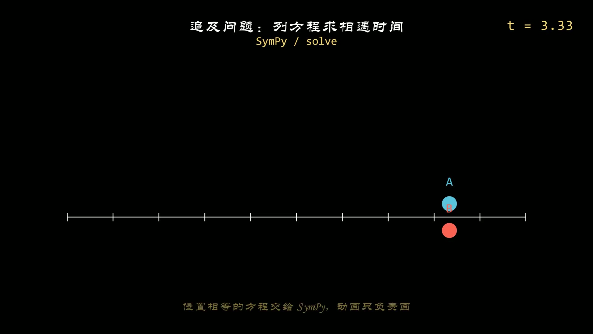
我们在做数学公式推导的视频时,比如,想展示一个因式分解:x2+2x+1 变成 (x+1)2 的,或者反过来因式展开,都需要手动计算分解或展开后的结果。
然后再做一个切换动画。
1
2
3
4
| from manim import *
expr1 = MathTex("x^2 + 2x + 1")
expr2 = MathTex("(x + 1)^2")
self.play(Transform(expr1, expr2))
|
简单的公式可以手动去做,如果公式稍微复杂呢?比如:
- x3−6x2+11x−6 可分解成:(x−1)(x−2)(x−3)
- 2x3+4x2−30x 可分解成:2x(x−3)(x+5)
- … …
这几个公式就不是那么容易分解了,我们制作公式变换的数学动画,或者绘制函数图像时,肯定不想把时间花在这些数学推导上。
那么,把 SymPy 引进了 Manim 的动画制作中—— 一切都变了。
1. 痛点还原:手动推导
假设我们要展示从 (x+2)(x−3) 展开到 x2−x−6 的过程。
传统做法会这样写:
1
2
3
4
5
6
7
8
9
10
11
12
| from manim import *
expr_origin = MathTex("(x + 2)(x - 3)")
expr_result = MathTex("x^2 - x - 6")
self.play(Transform(expr_origin, expr_result))
|
问题显而易见:
- 容易算错(特别是系数复杂时)
- 无法自动化(换个新公式就得重写代码)
- 缺乏动态生成的灵活性
我们真正需要的是一个能自动处理代数变形,并且把结果无缝喂给 Manim 的管道。
2. SymPy 登场:代数变形的“发动机”
SymPy 是 Python 的符号计算库,简单说就是能让计算机帮你推导数学公式。
核心武器:expand() 和 factor()
1
2
3
4
5
6
7
8
9
10
11
12
13
14
15
| from manim import *
from sympy import symbols, expand, factor, latex
x = symbols("x")
expr_factored = (x + 2) * (x - 3)
expr_expanded = expand(expr_factored)
print(expr_expanded)
expr_back = factor(expr_expanded)
print(expr_back)
|
expand() 方法可以帮助我们将因式展开;
factor() 方法则是分解因式。
SymPy 不仅能返回计算结果,还能生成 LaTeX 字符串,这正是 Manim 渲染公式需要的格式:
1
2
3
4
5
| from manim import *
from sympy import latex
latex_code = latex(expr_expanded)
print(latex_code)
|
有了这个“发动机”,我们只需要告诉 SymPy 起点和终点,中间的所有代数变形它都能自动计算。
3. Manim 联动实战:让公式自动推导
下面通过一个曲线绘制的示例来演示 SymPy 如何让 Manim 动画更加简单。
为了能够绘制曲线的方法能够通用,我们封装几个函数:
1
2
3
4
5
6
7
8
9
10
11
12
13
14
15
16
17
18
19
20
21
22
23
24
25
26
27
28
29
30
31
32
33
34
35
36
37
38
39
40
41
42
43
44
45
46
47
48
49
50
51
52
53
54
55
56
57
58
59
60
61
62
63
64
65
66
67
68
69
70
71
72
73
74
75
76
77
78
79
80
81
| from manim import *
from sympy import symbols, sympify, solve, Eq, latex, lambdify
def plot_function_curve(axes, equation_str, x_range, plot_range):
"""
绘制函数曲线
Args:
axes: 坐标系对象
equation_str: 方程字符串,如 "x**2 - x - 6"
x_range: 绘图 x 范围,如 [-3.5, 4.5]
plot_range: 用于 sympy 求解的 x 范围
Returns:
graph: 曲线对象
graph_label: 曲线标签
"""
x = symbols("x")
expr = sympify(equation_str)
f = lambdify(x, expr, modules="numpy")
graph = axes.plot(f, x_range=x_range, color=YELLOW, stroke_width=3)
graph_label = axes.get_graph_label(
graph, label=f"f(x)={latex(expr)}", x_val=x_range[1], direction=UP * 3
)
return graph, graph_label
def find_roots(equation_str):
"""
使用 SymPy 求解方程的根
Args:
equation_str: 方程字符串,如 "x**2 - x - 6"
Returns:
roots: 实数根列表
"""
x = symbols("x")
expr = sympify(equation_str)
solutions = solve(Eq(expr, 0), x)
roots = []
for sol in solutions:
if sol.is_real:
roots.append(float(sol))
return roots
def create_root_markers(axes, roots):
"""
创建零点标记和标签
Args:
axes: 坐标系对象
roots: 根的列表
Returns:
root_dots: 零点标记组
root_labels: 零点标签组
"""
root_dots = VGroup()
root_labels = VGroup()
for rx in roots:
dot = Dot(axes.c2p(rx, 0), color=RED, radius=0.1)
label = MathTex(f"({rx}, 0)", font_size=30, color=RED).next_to(dot, UP * 0.5)
root_dots.add(dot)
root_labels.add(label)
return root_dots, root_labels
|
下载 Python 脚本
其中:
plot_function_curve:根据曲线方程的字符串(比如"x**2 - x - 6")来绘制曲线find_roots:求解曲线方程的根,也就是和曲线和 X 轴的交点create_root_markers:把曲线方程的根标记出来
有了上面封装的函数,绘制一个曲线的动画代码就非常简洁了。
1
2
3
4
5
6
7
8
9
10
11
12
13
14
15
16
17
18
19
20
21
| from manim import *
import numpy as np
import sympy as sp
def head(cn, en):
t = Text(cn, font="STLiti", font_size=27).to_edge(UP)
s = Text(en, font="Consolas", font_size=20, color=YELLOW).next_to(t, DOWN, buff=0.10)
return VGroup(t, s)
def foot(cn):
return Text(cn, font="STLiti", font_size=20, color=YELLOW).to_edge(DOWN)
class FormulaBasic(Scene):
def construct(self):
self.add(head("公式推导:平方和变完全平方", "TransformMatchingTex"))
a = MathTex("x^2", "+2x", "+1").scale(1.3)
b = MathTex("(x+1)", "^2").scale(1.3)
self.add(a)
self.wait(0.6)
self.play(TransformMatchingTex(a, b), run_time=2.4)
self.wait(1.2)
self.play(b.animate.set_color(YELLOW), run_time=1.0)
self.play(FadeIn(foot("相同子串自动配对,其余部分做形变")), run_time=0.4)
self.wait(1.2)
|
上面的代码看着长,其实关键的就一行:equation = "x**2 - x - 6"。
其他部分都是渲染坐标系,创建各种元素的动画等等。
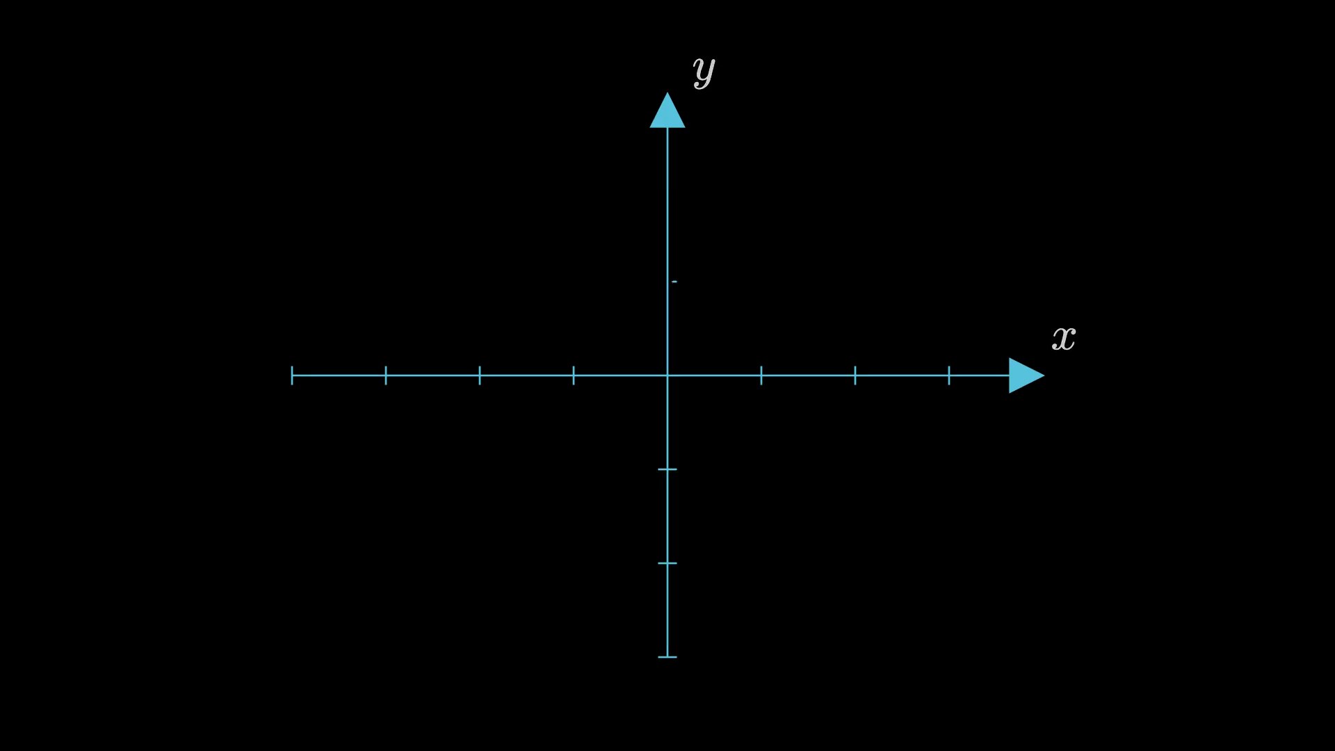
生成的效果如下:
下载 Python 脚本
使用 SymPy 中核心的几个方法如下:
sympify:比如,expr = sympify(equation_str)将曲线方程的字符串转换成 SymPy 中的符号公式lambdify:SymPy 中的符号公式转换为 Python 函数(供 Manim 绘制曲线用)latex:比如,latex(expr),将SymPy 中的符号公式转换为 Manim 中显示公式的 Latex 格式solve:solve(Eq(expr, 0), x),求解方程的根,也就是动画中标记的与 X 轴的交点
只从上面示例中的代码,可能还看不出来上 SymPy 和 Manim 结合的威力。
这时候,如果我们还想绘制另一个曲线 x3−6x2+11x−6,那么,只要改一行代码就行了。
equation = "x**2 - x - 6" 改成 "x**3 - 6*(x**2) +11*x - 6"
1
2
3
4
5
6
7
8
9
10
11
12
13
14
15
16
17
18
19
20
21
22
23
24
| from manim import *
import numpy as np
import sympy as sp
def head(cn, en):
t = Text(cn, font="STLiti", font_size=27).to_edge(UP)
s = Text(en, font="Consolas", font_size=20, color=YELLOW).next_to(t, DOWN, buff=0.10)
return VGroup(t, s)
def foot(cn):
return Text(cn, font="STLiti", font_size=20, color=YELLOW).to_edge(DOWN)
class FormulaFactor(Scene):
def construct(self):
self.add(head("公式推导:SymPy 自动因式分解", "sp.factor / MathTex"))
x = sp.symbols("x")
expr = x**3 - 6*x**2 + 11*x - 6
fac = sp.factor(expr)
a = MathTex(sp.latex(expr)).scale(1.2)
b = MathTex(sp.latex(fac)).scale(1.2)
self.add(a)
self.wait(0.6)
self.play(TransformMatchingTex(a, b), run_time=2.6)
self.wait(1.0)
self.play(b.animate.set_color(GREEN), run_time=1.0)
self.play(FadeIn(foot("分解结果由 SymPy 算出,不需要手写")), run_time=0.4)
self.wait(1.2)
|
这里显示的有点重叠,我们可以根据曲线显示的情况,调整下坐标系或曲线参数的范围。
1
2
3
4
5
6
7
8
9
10
11
12
13
14
15
16
17
18
19
20
21
22
23
24
| from manim import *
import numpy as np
import sympy as sp
def head(cn, en):
t = Text(cn, font="STLiti", font_size=27).to_edge(UP)
s = Text(en, font="Consolas", font_size=20, color=YELLOW).next_to(t, DOWN, buff=0.10)
return VGroup(t, s)
def foot(cn):
return Text(cn, font="STLiti", font_size=20, color=YELLOW).to_edge(DOWN)
class FormulaExpand(Scene):
def construct(self):
self.add(head("公式推导:展开与回代", "sp.expand / TransformMatchingTex"))
x = sp.symbols("x")
src = sp.expand((2*x - 3) * (x + 5))
dst = (2*x - 3) * (x + 5)
a = MathTex(sp.latex(src)).scale(1.2)
b = MathTex(sp.latex(dst)).scale(1.2)
self.add(a)
self.wait(0.6)
self.play(TransformMatchingTex(a, b), run_time=2.4)
self.wait(1.0)
self.play(TransformMatchingTex(b, a), run_time=2.0)
self.play(FadeIn(foot("展开式与因式式之间可以双向切换")), run_time=0.4)
self.wait(0.8)
|
下载 Python 脚本
4. 小结
本文主要内容如下:
- 痛点认知:手动推导公式既低效又容易出错。
- SymPy 核心技能:
expand() 展开、factor() 因式分解、latex() 转换。
- Manim 联动套路:
SymPy 算 → LaTeX 转 → Manim 渲染。
任何代数方程的因式变化或曲线函数都可以自动化生成,我们可以把精力集中在动画节奏和视觉设计上。

主观感受,仅供参考。本文采用 本文采用 CC BY-NC-SA 4.0 许可 协议,
完整转载请注明来自
数学动画引擎。