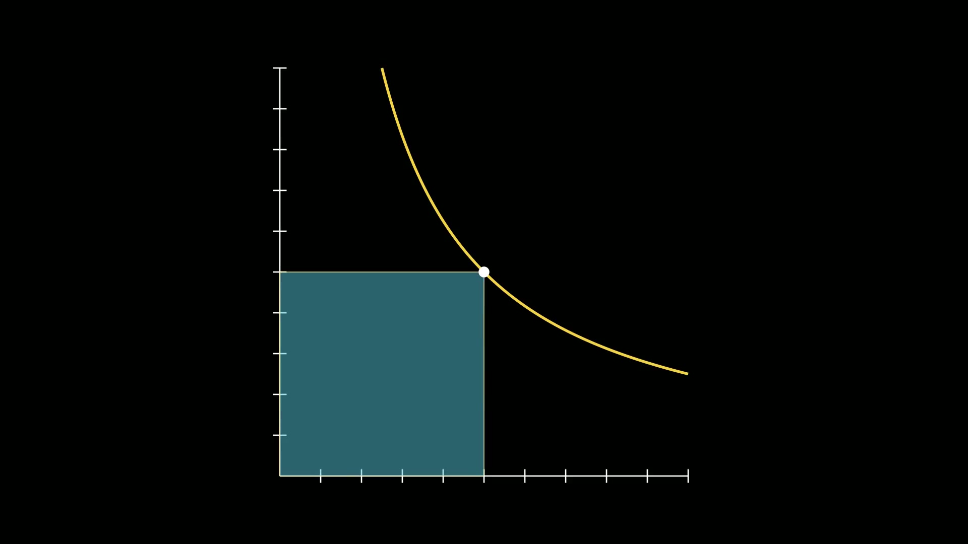
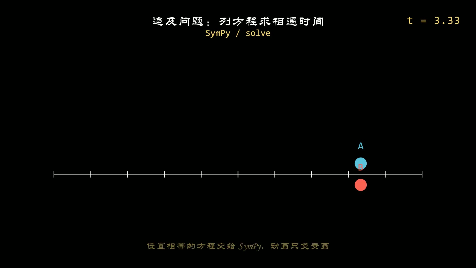
没有引入坐标系之前,在绘制图形时,也有一个隐含的坐标系,它和屏幕的像素相关。
比如,我们之前示例中的各个图形,屏幕的中心就是坐标原点([0, 0]),
横轴坐标的范围大概是 [-3.5, 3.5],纵轴的坐标范围大概是 [-4, 4],这个范围与设置的视频分辨率有关,分辨率设置的越高的话,坐标范围越大。
不知是否还记得,之前的文章中绘制的线或者多边形(比如这个系列第7篇),都是在上面的坐标范围的。
1
2
3
4
5
6
7
8
9
10
11
12
| from manim import *
class Demo(Scene):
def construct(self):
l = Line([-1, 0, 0], [1, 0, 0])
self.play(Create(l), run_time=0.5)
p = Polygon([-3, 1, 0], [-1, 1, 0], [-2, -1, 0])
self.play(Create(p), run_time=0.5)
p2 = Polygon([-4, 2, 0], [-1, 5, 0], [-2, -1, 0])
self.play(Create(p2), run_time=0.5)
self.wait(4.1)
|
下载 Python 脚本
引入坐标系之后,绘制图形时就不用局限在屏幕隐含的坐标范围之内,
通过调整坐标的刻度,我们可以基于坐标系中绘制任意范围的图形,而不用担心绘制到屏幕之外去。
manim已经提供了从一维到三维的坐标系对象,下面一一介绍它们的基本使用方法。
1. 数轴
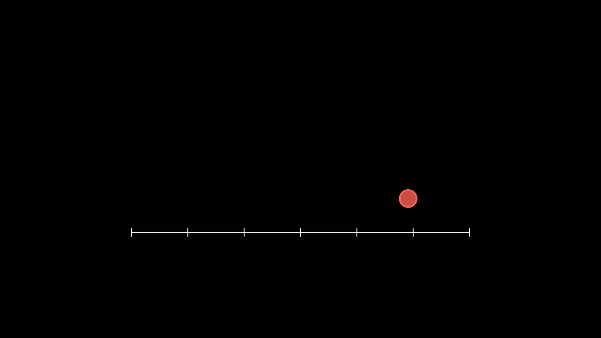
数轴(NumberLine)是最基本的一维坐标系,它的关键参数是:
x_range:设置数轴的范围和间隔length:设置数轴显示的长度
1
2
3
4
5
6
7
8
9
10
11
12
13
14
15
16
17
18
| from manim import *
import numpy as np
from numpy import array, pi, cos, sin
run_time = 1
data = [[1, 2], [3, 4]]
def dot(pos, **kwargs):
return Dot(pos, **kwargs)
class Z0038(Scene):
def construct(self):
sc = self
l = Line([-1, 0, 0], [1, 0, 0])
self.play(Create(l), run_time=0.5)
p = Polygon([-3, 1, 0], [-1, 1, 0], [-2, -1, 0])
self.play(Create(p), run_time=0.5)
p = Polygon([-4, 2, 0], [-1, 5, 0], [-2, -1, 0])
self.play(Create(p), run_time=0.5)
self.wait(0.5)
self.wait(3.60)
|
下载 Python 脚本
运行效果:
2. 平面坐标系
平面坐标系分为两类,实数平面和复数平面,两者的外形非常类似。
2.1 实数平面
实数平面(NumberPlane)的关键参数有4个:
- x_range:设置X轴的范围和间隔
- y_range:设置Y轴的范围和间隔
- x_length:设置X轴显示的长度
- y_length:设置Y轴显示的长度
1
2
3
4
5
6
7
8
9
10
11
12
13
14
15
| from manim import *
import numpy as np
from numpy import array, pi, cos, sin
run_time = 1
data = [[1, 2], [3, 4]]
def dot(pos, **kwargs):
return Dot(pos, **kwargs)
class Z0039(Scene):
def construct(self):
sc = self
self.play(*[FadeIn(_o) for _o in [NumberLine(x_range=[-10, 10, 2], length=10, include_numbers=True)]], run_time=1.0)
self.play(*[FadeIn(_o) for _o in [NumberLine(x_range=[-3, 3, 0.5], length=12, include_numbers=True)]], run_time=1.0)
self.play(*[FadeIn(_o) for _o in [NumberLine(x_range=[-5, 5 + 1, 1], length=6, include_numbers=True, include_tip=True, rotation=10 * DEGREES)]], run_time=1.0)
self.wait(0.5)
self.wait(2.10)
|
下载 Python 脚本
运行效果:
2.2 复数平面
复数平面(ComplexPlane)是基于实数平面(NumberPlane)的,参数类似,
只是多了一些标记复数的信息。
1
2
3
4
5
6
7
8
9
10
11
12
13
14
| from manim import *
import numpy as np
from numpy import array, pi, cos, sin
run_time = 1
data = [[1, 2], [3, 4]]
def dot(pos, **kwargs):
return Dot(pos, **kwargs)
class Z0040(Scene):
def construct(self):
sc = self
self.play(*[FadeIn(_o) for _o in [NumberPlane(x_range=(-4, 11, 1), y_range=(-3, 3, 1), x_length=3, y_length=2)]], run_time=1.0)
self.play(*[FadeIn(_o) for _o in [NumberPlane(x_range=(-4, 11, 1), x_length=3, y_length=4)]], run_time=1.0)
self.wait(0.5)
self.wait(3.10)
|
下载 Python 脚本
运行效果:
3. 极坐标系
极坐标系(PolarPlane)通过角度和与原点的距离来定位位置,经常被用于导航类的系统中,
与直角坐标相比,在这类系统中能极大的简化计算。
它的关键参数有:
- azimuth_step:分割的角度个数
- size:极坐标在屏幕中显示的大小
- radius_step:极坐标半径的间隔
- radius_max:极坐标最大半径
1
2
3
4
5
6
7
8
9
10
11
12
13
14
15
16
17
18
| from manim import *
class Demo(Scene):
def construct(self):
plane = PolarPlane(
azimuth_step=24,
size=6,
radius_step=1,
radius_max=3,
azimuth_units="PI radians",
azimuth_label_font_size=24,
background_line_style={"stroke_color": BLUE_B, "stroke_width": 2.5},
radius_config={"stroke_color": BLUE_B, "stroke_width": 2.5,
"include_ticks": True, "include_tip": False},
).add_coordinates()
plane.scale(1.15)
core = Dot(ORIGIN, color=BLUE_B, radius=0.08)
self.play(Create(plane), FadeIn(core), run_time=2.0)
self.wait(3.6)
|
下载 Python 脚本
运行效果:
下载 Python 脚本
4. 笛卡尔坐标系
笛卡尔坐标系是最常用的坐标系,学习函数的图像时用的最多的就是此坐标系。
4.1 二维
二维的笛卡尔坐标系(Axes)使用的比较多,它在平面坐标系之上,又提供了更多的配置,
可以更加灵活的配置数轴,除了上面平面坐标系提到的那4个关键参数之外,
还有2个配置坐标轴的参数也很重要:
- x_axis_config:配置X轴如何显示的参数
- y_axis_config:配置Y轴如何显示的参数
比如下面的示例中, 配置了与X轴不一样刻度的Y轴。
1
2
3
4
5
6
7
8
9
10
11
12
13
14
15
16
| from manim import *
class Demo(Scene):
def construct(self):
ax = Axes(
x_range=[0, 10, 1],
y_range=[-2, 6, 1],
x_length=6,
tips=False,
axis_config={"include_numbers": True},
y_axis_config={"scaling": LogBase(custom_labels=True)},
)
graph = ax.plot(lambda x: x**2, x_range=[0.001, 10], use_smoothing=False)
_obj = ax
self.play(FadeIn(_obj), run_time=1.0)
self.wait(3.00)
self.wait(1.60)
|
下载 Python 脚本
运行效果:
下载 Python 脚本
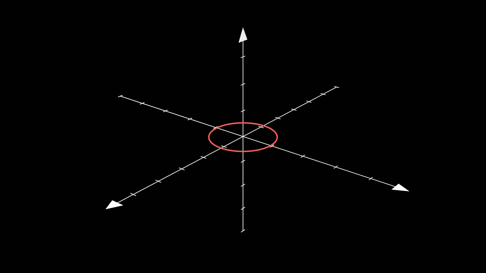
4.2 三维
三维的笛卡尔坐标系(ThreeDAxes)与二维坐标系的参数类似,只是多了一个维度(Z轴)的配置,
其配置参数与X轴和Y轴类似。
显示三维图形时,有2点需要额外注意,
一是场景要继承 ThreeDScene,二是要调整下默认的相机位置,也就是视角的位置,默认视角是从Z轴顶部向下看的。
1
2
3
4
5
6
7
8
| from manim import *
class Demo(ThreeDScene):
def construct(self):
axes = ThreeDAxes(y_length=8)
circle = Circle(color=BLUE, radius=2)
vg = VGroup(axes, circle)
self.play(Create(vg), run_time=2.0)
self.wait(3.6)
|
下载 Python 脚本
运行效果如下,很难看出是三维的坐标系统:
下载 Python 脚本
加入调整视角的代码后:
1
2
3
4
5
6
7
8
9
| from manim import *
class Demo(ThreeDScene):
def construct(self):
axes = ThreeDAxes(y_length=8)
circle = Circle(color=BLUE, radius=2)
vg = VGroup(axes, circle)
self.set_camera_orientation(phi=75 * DEGREES, theta=30 * DEGREES)
self.play(Create(vg), run_time=2.0)
self.wait(3.6)
|
下载 Python 脚本
修改后运行效果:
下载 Python 脚本
5. 总结回顾
本篇主要介绍各类坐标系的基本使用方式和常用参数,从一维到三维主要有以下几种坐标系对象:
- NumberLine:数轴
- NumberPlane:实数平面
- ComplexPlane:复数平面
- PolarPlane:极坐标系
- Axes:二维笛卡尔坐标系
- ThreeDAxes:三维笛卡尔坐标系
制作函数相关的数学动画,或者物理定律相关的动画时,借助坐标系可以更清晰直观的的表达变换的规律。

主观感受,仅供参考。本文采用 本文采用 CC BY-NC-SA 4.0 许可 协议,
完整转载请注明来自
数学动画引擎。